一起学习机器学习（13）：PCA 与 NMF

这组文章整理自 2024 年的课程学习笔记，保留原练习、代码和图表。运行前请先看系列目录中的环境与数据说明。查看系列目录。

Linear dimensionality reduction

The purpose of this notebook is to understand and implement two linear dimensionality reduction methods:

Principle component analysis (PCA)
Non-Negative Matrix Factorization (NMF)

The main idea of these methods is to approximate our data by a linear combination of a few components, which span the space for a low-dimensional representation of the data. Such representation is often useful to visualise and inspect the structure of the data in an easier way, allowing us to better understand their properties. Here we illustrate the application of PCA and NMF to a dataset of hand-written digits (MNIST).

# Imports in alphabetical order

import matplotlib.pyplot as plt
import numpy as np
import pandas as pd
import scipy
import random

from scipy.sparse import linalg
from sklearn.datasets import fetch_openml # we need this only to import a standard dataset in data science, the MNIST dataset

# Changing default font sizes
plt.rc('xtick', labelsize=16) # Tick labels
plt.rc('ytick', labelsize=16) # Tick labels
plt.rc('legend', fontsize=14) # Legend
plt.rc('axes', titlesize=24, labelsize=20) # Title and 'x' and 'y' labels

Let’s first load the data. We will use the MNIST dataset for this problem.

1
2
3

# Loading the images
images, labels = fetch_openml('mnist_784', version=1, return_X_y=True)
images = images.to_numpy()

# Plotting the second image
plt.figure(figsize=(4,4))
plt.xlabel('Pixel Index', size=14)
plt.ylabel('Pixel Index', size=14)
plt.title('Raw image', size=14)
plt.imshow(images[1].reshape(28,28), cmap='gray')
plt.colorbar();

请添加图片描述

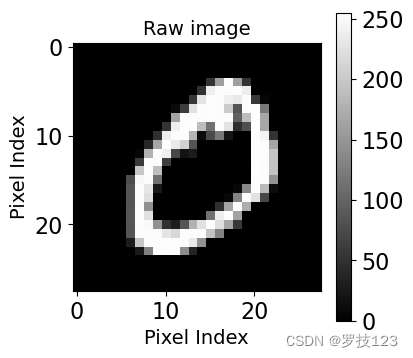
Let’s now pre-process the data.

The steps below ensure that our images will have zero mean and unitary variance. These pre-processing
steps are also known as data normalisation/standardisation or feature scaling.

The pre-processing steps are:

Converting an unsigned integer (u-int8) encoding each pixel to a floating point number between 0 and 1.
Subtracting from each pixel the mean $μ\boldsymbol \mu$ across pixels.
Scaling by $1σ\frac{1}{\sigma}$ where $σ\sigma$ is the stardard deviation.

# Pre-processing

# We consider the first 500 images
n_datapoints = 500

# Reshaping and taking a slice of the data
X = (images.reshape(-1, images.shape[-1])[:n_datapoints]) / 255.

## EDIT THIS FUNCTION

def standardise(X):
    """
    Arguments:
    X: Data with samples being indexed along axis 0.

    Returns:
    Xbar: Standardised data.

    """
    mu = np.mean(X, axis=0) # <-- SOLUTION
    std = np.std(X, axis=0) # <-- SOLUTION
    std[std==0] = 1. # <-- SOLUTION
    Xbar = (X - mu) / std # <-- SOLUTION

    return Xbar

1 2	X_norm = standardise(X) X_norm.shape

1	(500, 784)

# Plotting the second image (now standardised)
plt.figure(figsize=(4,4))
plt.xlabel('Pixel Index', size=14)
plt.ylabel('Pixel Index', size=14)
plt.title('Standardised image', size=14)
plt.imshow(X_norm[1].reshape(28,28), cmap='gray')
plt.colorbar();

请添加图片描述

1
2
3

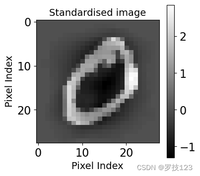
# Let's verify that a given pixel across all the images now has zero mean and unitary standard deviation
np.testing.assert_allclose(np.std(X_norm[:, 300]), 1)
np.testing.assert_allclose(np.mean(X_norm[:, 300]+0.001), 0.001) # Note that if we do not add a small number like 0.001 this does not work

1. PCA

Now we will implement PCA. Before we do that, let’s pause for a moment and
think about the steps for performing PCA. Assume that we are performing PCA on
some dataset $X\mathbf{X}$ for $k$ principal components.
We then need to perform the following steps, which we break into parts:

Compute the covariance matrix $C\mathbf C$ .
Find eigenvalues and corresponding eigenvectors for the covariance matrix, $C=VLV⊤\mathbf C = \mathbf V \mathbf L \mathbf V^\top$ . The matrix $V\mathbf{V}$ is composed of the eigenvectors of matrix $C\mathbf{C}$ as its columns, while $L\mathbf{L}$ is a diagonal matrix with the eigenvalues of $C\mathbf{C}$ as its diagonal elements.
Sort by the largest eigenvalues and the corresponding eigenvectors.
Compute the projection onto the spaced spanned by the top eigenvectors.

## EDIT THIS FUNCTION

def covariance_matrix(X):
    """
    Arguments:
    X: Data with samples being indexed along axis 0.

    Returns:
    Xbar: Computes the data covariance matrix.

    """
    return np.dot(X.T, X) / len(X) # <-- SOLUTION

def pca_function(X, k):
    """
    Arguments:
    X: Data with samples being indexed along axis 0.
    k: Number of principal components.

    Returns:
    X_pca: Transformed data.
    eigenvectors: First k eigenvectors of C.
    eigenvalues: First k eigenvalues of C.

    """
    # Computing the covariance matrix
    C = covariance_matrix(X)

    # Computing the eigenvalues and eigenvectors using the eigsh scipy function
    eigenvalues, eigenvectors = linalg.eigsh(C, k, which='LM', return_eigenvectors=True) # <-- SOLUTION

    # Sorting the eigenvectors and eigenvalues from largest to smallest eigenvalue
    sorted_index = np.argsort(eigenvalues)[::-1] # <-- SOLUTION
    eigenvalues = eigenvalues[sorted_index] # <-- SOLUTION
    eigenvectors = eigenvectors[:,sorted_index] # <-- SOLUTION

    # Projecting the data onto the directions of eigenvectors
    X_pca = X.dot(eigenvectors) # <-- SOLUTION

    return X_pca, eigenvectors, eigenvalues

Test the PCA function for three principal components ( $k = 3$ ) and print the eigenvalues.

k = 3 # Our number of principal components

X_pca, eigenvectors, eigenvalues = pca_function(X_norm, k)
print(eigenvalues)

np.testing.assert_allclose(eigenvalues, np.array([45.28147173, 30.46538702, 27.12873262]))

1	[45.28147173 30.46538702 27.12873262]

Now consider a larger number such as $k = 100$ . Plot the spectrum, i.e., the histogram of the eigenvalues of $C\mathbf{C}$ with the density parameter set to True.

k = 100
X_pca, eigenvectors, eigenvalues = pca_function(X_norm, k)

# If we look at the spectrum, the large values indicate there is some signal of significant correlations

plt.hist(eigenvalues, density=True);
plt.xlabel('Eigenvalues of $C$')
plt.ylabel('Density')
plt.show()

请添加图片描述

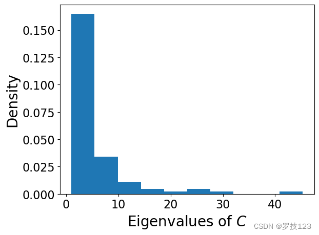
If we randomly permute the pixels of each image, which is equivalent to ‘randomising’ the data, the large eigenvalues disappear. Reshuffle every column separately to remove correlations between pixels

X_norm_random = np.copy(X_norm)

for n in range(X_norm.shape[1]): # <-- SOLUTION
    permutation = random.sample(list(np.arange(X_norm.shape[0])), X_norm.shape[0]) # <-- SOLUTION
    X_norm_random[:, n] = X_norm[:, n][permutation] # <-- SOLUTION

# The spectrum of eigenvalues this 'random' matrix has not large values!

X_norm_random = standardise(X_norm_random)
X_pca_random, eigenvectors_random, eigenvalues_random = pca_function(X_norm_random, k)

plt.hist(eigenvalues_random, density=True);
plt.xlabel('Eigenvalues of C')
plt.ylabel('Density')
plt.show()

请添加图片描述

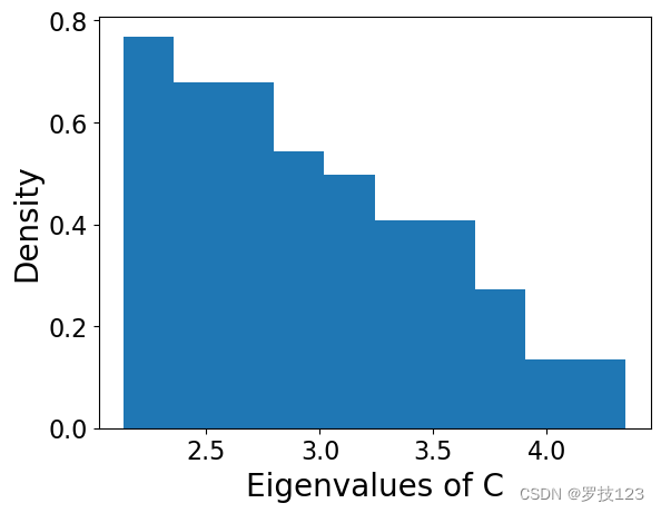
Question: what can you say about the previous plot? Compare it with the case in which the columns were not randomly permuted ( $k = 100$ ).

Let’s go back to the original case with $k = 100$ and analyse what fraction of the overall variance is explained by the components.

C = covariance_matrix(X_norm)
all_eigenvalues, _ = np.linalg.eig(C) # <-- SOLUTION
total_variance = abs(all_eigenvalues.sum()) # <-- SOLUTION

explained_variances = [abs(eigenvalues[:j].sum()) / total_variance for j in range(k)] # <-- SOLUTION

plt.plot(np.arange(k), explained_variances)
plt.axhline(y = 1, color = 'r', linestyle = '-', label='Full variance')
plt.axhline(y = 0.8, color = 'k', linestyle = '--', label='80% of variance')
plt.xlabel('Eigenvalue Index')
plt.ylabel('Fraction of Captured Variance')
plt.legend()
plt.show()

np.testing.assert_allclose(explained_variances[64], 0.803337909682404)

请添加图片描述

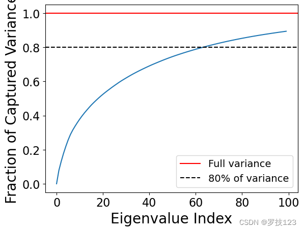
Find the number of components that allows us to explain at least 80% of the total variance.

1 2	opt_k = np.argmax(np.array(explained_variances) >= 0.8) # <-- SOLUTION opt_k

Let’s now try and understand what these different principle components represent for a given image. Plot the first 20 eigenvectors as images.

nrow = 5; ncol = 4; # <-- SOLUTION
fig, axs = plt.subplots(nrows=nrow, ncols=ncol, figsize=(13,19)) # <-- SOLUTION

for i, ax in enumerate(axs.reshape(-1)): # <-- SOLUTION
    ax.imshow(eigenvectors[:,i].reshape([28,28])) # <-- SOLUTION
    ax.set_title('Component '+str(i), size=16) # <-- SOLUTION

请添加图片描述

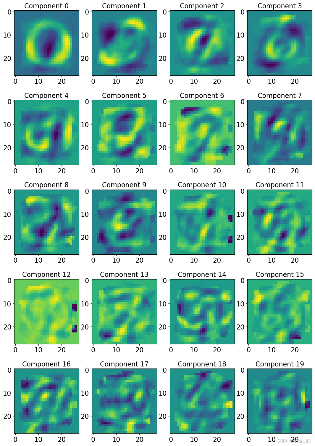
Using opt_k principal components, try to approximate the image of index_image equal to 5.

index_image = 5

# We represent each image as a linear combination of principal components
approximate_image = 0 # <-- SOLUTION
for y in range(opt_k): # <-- SOLUTION
    approximate_image += X_pca[index_image,y] * eigenvectors[:,y] # <-- SOLUTION

fig, ax = plt.subplots(2, 1, figsize=(10,10))
ax[0].imshow(X_norm[index_image].reshape([28,28]))
ax[0].set_title('Original Image')
ax[1].imshow(approximate_image.reshape([28,28]))
ax[1].set_title('Approximated Image');

请添加图片描述

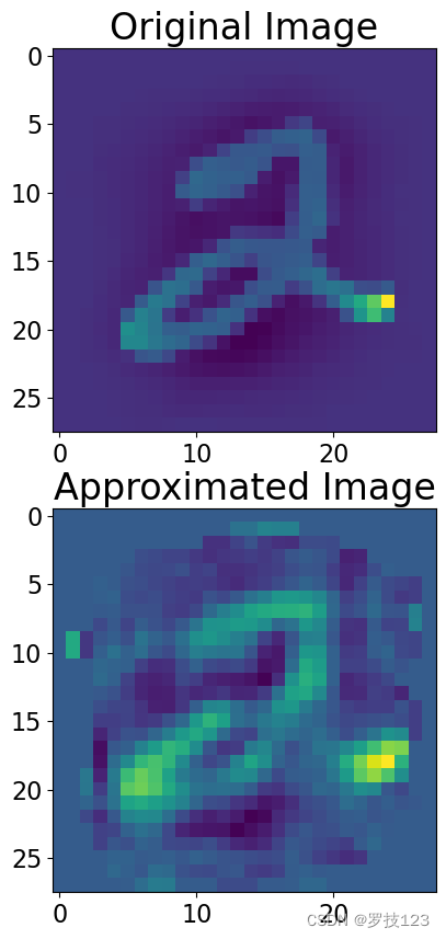
Exercise: compute the estimated image using $k$ components that account for $70$ and $90%90\%$ of the total variance.

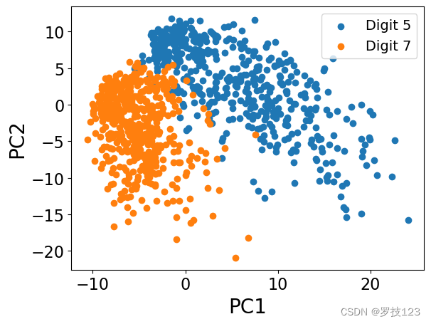
Consider now digits 5 and 7 only, and the first two principal components. Plot the data points in a 2D space based on their projections onto eigenvectors 1 and 2 (PC1 and PC2).

ind_5 = [i for i in range(len(labels)) if labels[i] == '5'] # <-- SOLUTION
ind_7 = [i for i in range(len(labels)) if labels[i] == '7'] # <-- SOLUTION
X_5 = (images.reshape(-1, images.shape[-1])[ind_5[:n_datapoints]]) / 255. # <-- SOLUTION
X_7 = (images.reshape(-1, images.shape[-1])[ind_7[:n_datapoints]]) / 255. # <-- SOLUTION
X = np.vstack((X_5, X_7)) # <-- SOLUTION

k = 2
X_norm = standardise(X)
X_pca, eigenvectors, eigenvalues = pca_function(X_norm, k)

plt.scatter(X_pca[:n_datapoints, 0], X_pca[:n_datapoints, 1], label='Digit 5')
plt.scatter(X_pca[n_datapoints:X.shape[0], 0], X_pca[n_datapoints:X.shape[0], 1], label='Digit 7')
plt.legend()
plt.xlabel('PC1')
plt.ylabel('PC2');

请添加图片描述

Exercise:

Define an error between the original and the approximated image. A standard choice is the Mean Squared Error (MSE).
Calculate the MSE for all images.
Plot the average MSE as a function of $k$ . Can we use this plot to decide opt_k?

2. NMF

Now we will look at non-negative matrix factorisation. NMF is a matrix factorisation method where we constrain the matrices to have nonnegative elements (while PCA produces components with elements that could be both positive and negative).

NMF factors our N-by-p data matrix $X\mathbf X$ into matrices with nonnegative elements $W\mathbf W$ (N-by-r) and $H\mathbf H$ (r-by-p), i.e. $X∼WH\mathbf X \sim \mathbf W\mathbf H$ . $WH\mathbf W\mathbf H$ is lower-rank ( $r < p$ ), hence it gives a low-dimensional approximation of $X\mathbf X$ .

Note that for non-negative matrix factorisation we require the input matrix to be non-negative. Therefore, we must normalise between 0 and 1 instead of the standard normalisation which we used for PCA.

## EDIT THIS FUNCTION

# normalise min max to 0-1
def normalize_nmf(X):
    X_norm = (X- np.min(X)) / (np.max(X) - np.min(X)) ## <-- SOLUTION
    return X_norm

1	print("Min:",np.min(X), "and max:",np.max(X))

1	Min: 0.0 and max: 1.0

## Redefine the matrix X before applying a new normalization ##

# we take the first 1000 images
n_datapoints = 1000

# reshaping and taking a slice of the data
X = (images.reshape(-1, images.shape[-1])[:n_datapoints]) / 255.

Xn = normalize_nmf(X)

As explained in the lecture notes, we find $W$ and $H$ as the local minima of cost functions that represent the quality of the approximation of $X$ by $W H$ . We will see the implementation of the optimisation of the two main cost functions used for NMF.

The first is the square of the Euclidean distance between the data $X$ and the product $W H$ :

$
||\mathbf{X} - \mathbf{WH}||^2 = \sum_{ij}(X_{ij} - (\mathbf{WH})_{ij})^2
$

Local minima of this function are found by the Lee and Seung’s multiplicative update rules

$
H_{jk}^{n+1}\leftarrow H_{jk}^{n}
\frac{(( \mathbf{W}^n)^T \mathbf{X}){jk}}{((\mathbf{W}^n)^T \mathbf{W}^n \mathbf{H}^n){jk}}
$

and

$
W_{ij}^{n+1}\leftarrow W_{ij}^{n}
\frac{(\mathbf{X}(\mathbf{H}^{n+1})^T){ij}}{(\mathbf{W}^n \mathbf{H}^{n+1} (\mathbf{H}^{n+1})^T){ij}}
$

which are repeated for several iterations $n$ until $W\mathbf{W}$ and $H\mathbf{H}$ converge. It is important to note that updates are done on an element by element basis and not by matrix multiplication.

## EDIT HERE

# lets define a cost matrix to compare the difference
def cost(X,W,H):

    """
    Arguments:
    X: Data with range [0,1].
    W, H: factorisation of X

    Returns:
    cost_value: (component-wise) squared Euclidean distance between X and WH

    """

    # Check that W and H can be multiplied together
    assert W.shape[1] == H.shape[0], "The inner dimensions of W and H do not match for multiplication."

    # Test to see whether the size of X and the size of W times H matches
    assert X.shape == (W.shape[0], H.shape[1]), "The dimensions of X do not match the dimensions of WH."

    # compute the difference between X and the dot product of W and H
    diff = X - np.dot(W, H) ## <-- SOLUTION

    # Compute the Euclidean distance-based objective function
    cost_value = (diff * diff).sum() / (X.shape[0]*X.shape[1]) ## <-- SOLUTION

    # Here we have also normalised the sum by the nummber of terms in the sum (but it's not necessary).

    return cost_value

Now implement Lee and Seung’s multiplicative update rule. First implement the update on H and then the update on W, finally compute the objective function.

# choosing the number of dimensions (r) on which to project
r = 2

# setting the random seed (just so everyone gets the same results...)
np.random.seed(0)

# r x P matrix interpreted as the basis set, where r is the number of components, P the number of descriptors of the data
H = np.random.rand(r, Xn.shape[1])

# N x r components matrix, usually interpreted as the coefficients, N is the number of data
W = np.random.rand(X.shape[0], r)

# set the number of iterations
n_iters = 500
epsilon = 0.001 ## this is just a small value that we place at the denominator to avoid division by zero

# empty list
cost_values = []

# loop over the n iterations
for i in range(n_iters):

    # compute the update on H
    H = H * ((W.T.dot(Xn))/(W.T.dot(W.dot(H))+epsilon)) ## <-- SOLUTION

    # compute the update on W
    W = W * ((Xn.dot(H.T))/(W.dot(H.dot(H.T))+epsilon)) ## <-- SOLUTION

    # compute the cost and append to list
    cost_values.append(cost(Xn,W,H))

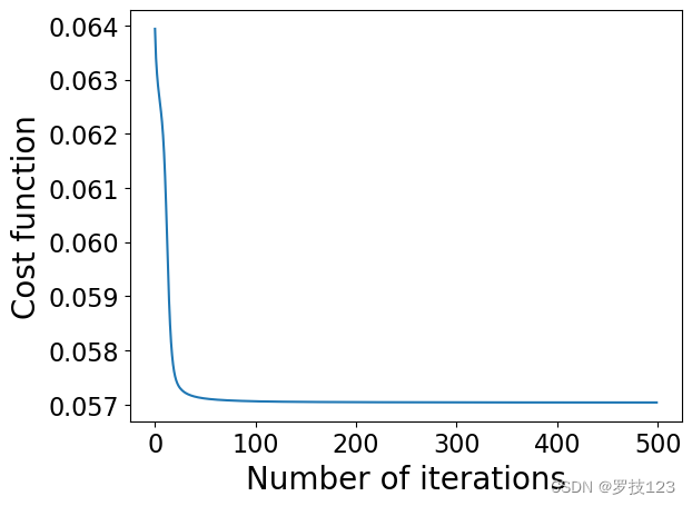
1	np.testing.assert_allclose(cost_values[-1], 0.057035312210066795)

We should next check to confirm that we have converged to a solution by plotting the value of our objective function over the iterations.

# plotting the cost, to check convergence
plt.plot(cost_values)
plt.xlabel('Number of iterations')
plt.ylabel('Cost function')
plt.show()

请添加图片描述

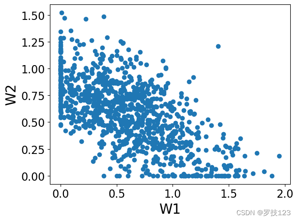
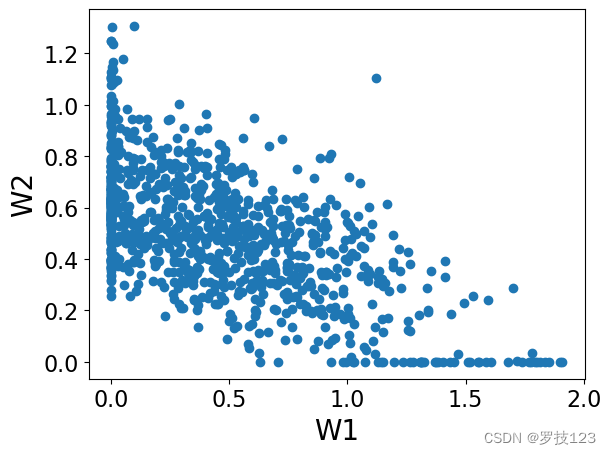
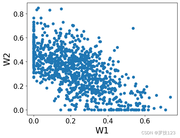
plt.scatter(W[:,0],W[:,1])
plt.xlabel('W1')
plt.ylabel('W2')
plt.show()

请添加图片描述

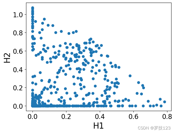
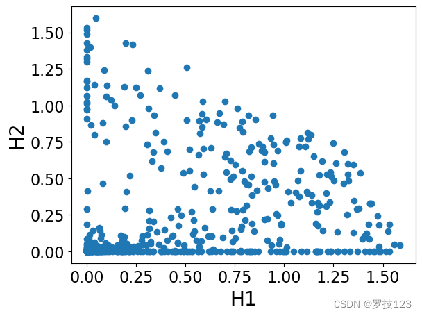
plt.scatter(H[0,:],H[1,:])
plt.xlabel('H1')
plt.ylabel('H2')
plt.show()

请添加图片描述

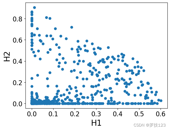
We can observe that these matrices have non-negative entries as we expected, and also they are sparse (which is a desirable property!).

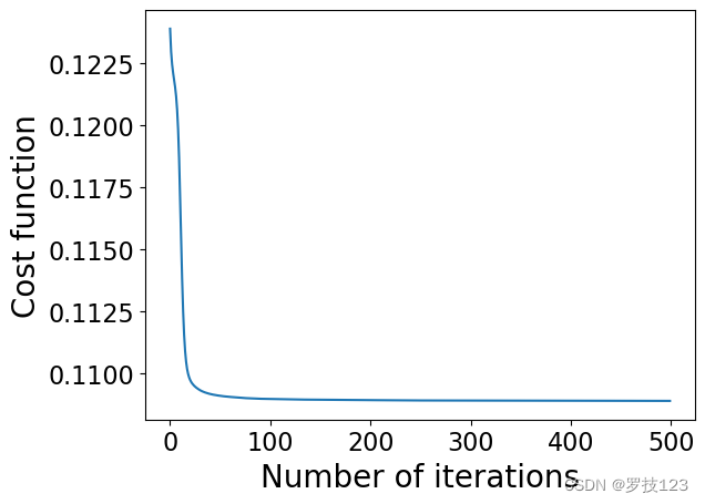
We can see above that we have converged in optimising our NMF according to the Euclidean distance objective function. Next, we repeat the optimisation monitoring the trend of a different objective function, the divergence $D$ defined as:

$
D(\mathbf{X}||\mathbf{WH}) = \sum_{ij}\left[X_{ij} \log\left(\frac{X_{ij}}{(\mathbf{WH}){ij}}\right) - X{ij} +(\mathbf{WH})_{ij}\right]
$

for which we are guaranteed to find local minima by slightly different multiplicative update rules:

$
H_{jk}^{n+1}\leftarrow H_{jk}^{n}
\frac{ \sum_i W^n_{ij}X_{ik} / (\mathbf{W}^n\mathbf{H}^n){ik}}{\sum_i W^n{ij}}
$

and

$
W_{ij}^{n+1}\leftarrow W_{ij}^{n}
\frac{\sum_k H_{jk}X_{ik} / (\mathbf{W}^n\mathbf{H}^{n+1}){ik} }{\sum_k H^{n+1}{jk}}
$

## EDIT HERE

# lets define a cost matrix to compare the difference
def cost(X,W,H):

    """
    Arguments:
    X: Data with range [0,1].
    W, H: factorisation of X

    Returns:
    cost_value: divergence between X and WH

    """

    # Check that W and H can be multiplied together
    assert W.shape[1] == H.shape[0], "The inner dimensions of W and H do not match for multiplication."

    # Test to see whether the size of X and the size of W times H matches
    assert X.shape == (W.shape[0], H.shape[1]), "The dimensions of X do not match the dimensions of WH."


    ## we add a small epsilon to avoid ill-defined divisions/log
    epsilon1 = 0.0001

    # compute the divergence term by term
    term = X*np.log(np.divide(X,np.dot(W, H)+ epsilon1) + epsilon1) - X + np.dot(W, H)  ## <-- SOLUTION

    # sum over the terms
    cost_value = term.sum()/ (X.shape[0]*X.shape[1]) ## <-- SOLUTION
    # Here we have also normalised the sum by the nummber of terms in the sum (but it's not necessary).

    return cost_value

# choosing the number of dimensions (r) on which to project
r = 2

# setting the random seed (just so everyone gets the same results...)
np.random.seed(0)

# r x P matrix interpreted as the basis set, where r is the number of components, P the number of descriptors of the data
H = np.random.rand(r, Xn.shape[1])

# N x r components matrix, usually interpreted as the coefficients, N is the number of data
W = np.random.rand(Xn.shape[0], r)

# set the number of iterations
n_iters = 500
epsilon = 0.0001 ## this is just a small value that we place at the denominator to avoid division by zero

# empty list
cost_values = []

# loop over the n iterations
for i in range(n_iters):

    # compute the update on H
    H = H * ((W.T.dot(Xn/(W.dot(H)+epsilon))/(W.T.dot(np.ones_like(Xn))) + epsilon)) ## <-- SOLUTION

    # compute the update on W
    W = W * (((Xn/(W.dot(H)+epsilon)).dot(H.T))/(np.ones_like(Xn).dot(H.T) + epsilon)) ## <-- SOLUTION

    # compute the cost and append to list
    cost_values.append(cost(Xn,W,H))

1	np.testing.assert_allclose(cost_values[-1], 0.10888229870847117)

# plotting the cost, to check convergence
plt.plot(cost_values)
plt.xlabel('Number of iterations')
plt.ylabel('Cost function')
plt.show()

请添加图片描述

plt.scatter(W[:,0],W[:,1])
plt.xlabel('W1')
plt.ylabel('W2')
plt.show()

请添加图片描述

plt.scatter(H[0,:],H[1,:])
plt.xlabel('H1')
plt.ylabel('H2')
plt.show()

请添加图片描述

As an exercise, you can check that the result of NMF is the same if you
use another version of cost function, the one from the paper:
https://www.nature.com/articles/44565.

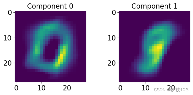
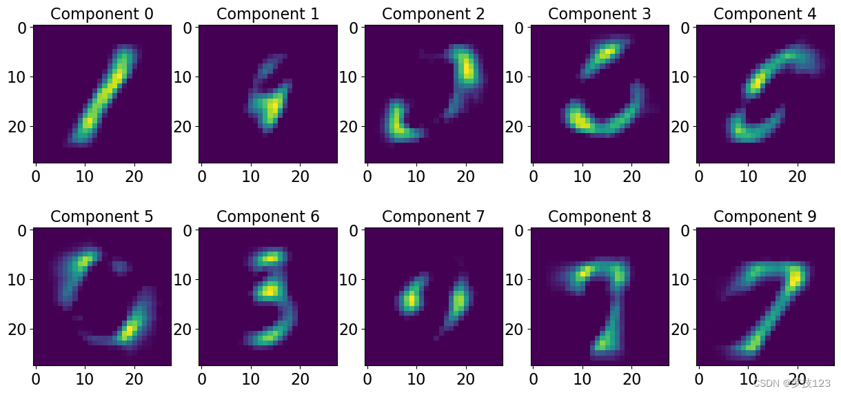
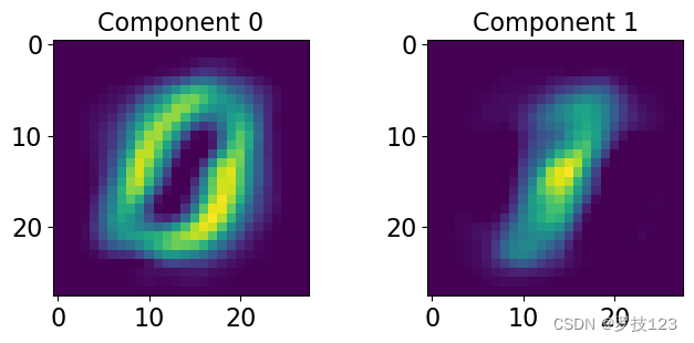
Finally, we can have a look at the difference components resulting from our NMF and see what information they might contain.

nrow = 1; ncol = 2; # <-- SOLUTION
fig, axs = plt.subplots(nrows=nrow, ncols=ncol, figsize=(8,3)) # <-- SOLUTION

for i, ax in enumerate(axs.reshape(-1)): # <-- SOLUTION
    ax.imshow(H[i,:].reshape([28,28])) # <-- SOLUTION
    ax.set_title('Component '+str(i), size=16) # <-- SOLUTION

请添加图片描述

Try another value of r.

# choosing the number of dimensions (r) on which to project
r = 10

# setting the random seed (just so everyone gets the same results...)
np.random.seed(0)

# r x P matrix interpreted as the basis set, where r is the number of components, P the number of descriptors of the data
H = np.random.rand(r, Xn.shape[1])

# N x r components matrix, usually interpreted as the coefficients, N is the number of data
W = np.random.rand(Xn.shape[0], r)

# set the number of iterations
n_iters = 500
epsilon = 0.0001 ## this is just a small value that we place at the denominator to avoid division by zero

# empty list
cost_values = []

# loop over the n iterations
for i in range(n_iters):

    # compute the update on H
    H = H * ((W.T.dot(Xn/(W.dot(H)+epsilon))/(W.T.dot(np.ones_like(Xn))) + epsilon)) ## <-- SOLUTION

    # compute the update on W
    W = W * (((Xn/(W.dot(H)+epsilon)).dot(H.T))/(np.ones_like(Xn).dot(H.T) + epsilon)) ## <-- SOLUTION

    # compute the cost and append to list
    cost_values.append(cost(Xn,W,H))

1	np.testing.assert_allclose(cost_values[-1], 0.07084365237320929)

nrow = 2; ncol = 5; # <-- SOLUTION
fig, axs = plt.subplots(nrows=nrow, ncols=ncol, figsize=(15,7)) # <-- SOLUTION

for i, ax in enumerate(axs.reshape(-1)): # <-- SOLUTION
    ax.imshow(H[i,:].reshape([28,28])) # <-- SOLUTION
    ax.set_title('Component '+str(i), size=16) # <-- SOLUTION

请添加图片描述

We can now do this using sklearn and check that our methodology was implemented correctly. We expect this to be slightly different, the sklearn implementation relies on the optimisation of a slightly different objective function:
https://scikit-learn.org/stable/modules/generated/sklearn.decomposition.NMF.html

r = 2
from sklearn.decomposition import NMF
nmf = NMF(n_components=r, init='random', random_state=1)
W = nmf.fit_transform(Xn)
plt.scatter(W[:,0],W[:,1])
plt.xlabel('W1')
plt.ylabel('W2')
plt.show()

请添加图片描述

H = nmf.components_
plt.scatter(H[0,:],H[1,:])
plt.xlabel('H1')
plt.ylabel('H2')
plt.show()

请添加图片描述

nrow = 1; ncol = 2; # <-- SOLUTION
fig, axs = plt.subplots(nrows=nrow, ncols=ncol, figsize=(8,3)) # <-- SOLUTION

for i, ax in enumerate(axs.reshape(-1)): # <-- SOLUTION
    ax.imshow(H[i,:].reshape([28,28])) # <-- SOLUTION
    ax.set_title('Component '+str(i), size=16) # <-- SOLUTION